Optimizing Prediction-Target Assignments via Hungarian Matcher
4 February 2025In 2020, Carion et al. introduced an end-to-end method for object detection in images using transformers, enabling robust object detection without relying on hand-crafted methods like anchor boxes or NMS. It formulates the problem as a set prediction task, in which we directly estimate the bounding boxes of detected objects.
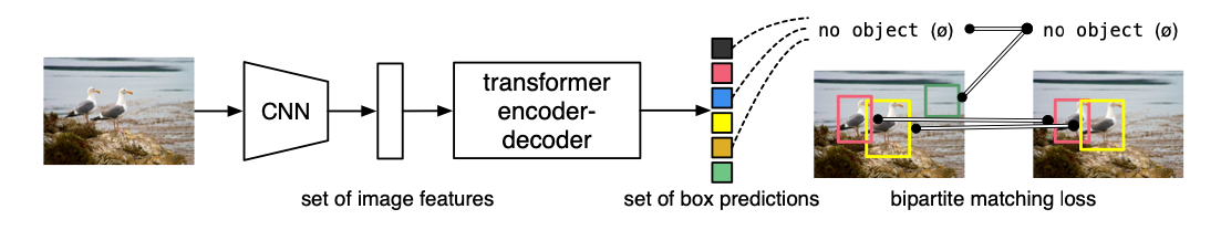 DETR combines a CNN with transformers to generate object detections directly in parallel. It leverages bipartite matching to pair predictions with ground truth boxes.
To select the best matches for each object, it uses Hungarian matching to solve this assignment problem. While it has its own limitations, the approach has proven useful for specific use cases. In 2022, Wolf et al. demonstrated that adapting this approach to work on time series data yields satisfactory results for segmenting EEG data for ocular event detection.
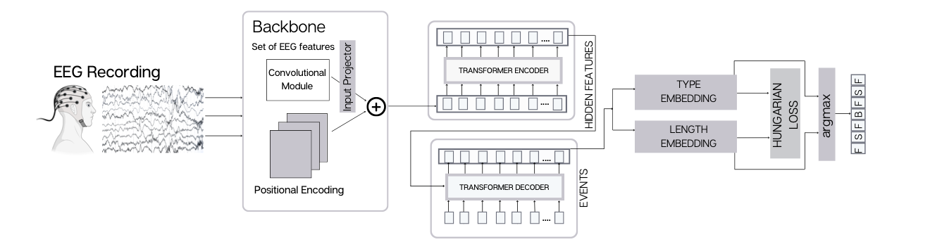 DETRtime Architecture
For the purposes of my current project, I am interested in how this object matching exactly works and how to extend / modify this technique to support scenarios of complete scanpath prediction.
Optimal Assignment
When training machine learning models that generate structured outputs like as object detection models or event segmentation models, it can be tricky to correctly assign predicted outputs to ground truth targets. Consider a typical classification problem: each predicted output corresponds to a specific class, and we can directly compute the loss for each prediction. But what if our model produces multiple structured outputs, such as bounding boxes in object detection or event segments in time series analysis? The number of predicted objects doesn’t necessarily match the number of ground truth objects, and their order is arbitrary. Unlike classification, where each output has a fixed position, we first need figure out how they correspond to each other before we can compute a meaningful loss.
For example, in object detection, a model might predict 100 bounding boxes, but there might only be 5 actual objects in the image. Some predictions are useful, some should be ignored, and some ground truth objects may have multiple candidates. Which prediction should correspond to which ground truth object? And how do we compute a meaningful loss for them?
The Hungarian Algorithm is a method that can be used to solve an assignment problem by finding the optimal matching in a bipartite graph. Consider the following problem as an example of an assignment problem.
There are three workers A,B and C offering services (jobs) X,Y and Z at different prices. You need all 3 services but one worker can only be hired to do one job. How do we get the optimal assignment of the services to the companies such that your cost is minimized?
Generally we are trying to model assignment between two groups of objects. In this context following the example, we call the vertices in set $U$ “workers” and vertices from group $V$ “jobs”. can This can be modelled as a matrix and as a bipartite graph $G = (U,V,E,w)$, where:
- $U$ and $V$ desciribing the two disjoint sets of objects (workers and jobs)
- $E \subseteq U \times V$ is the set of edges connecting vertices in $U$ to vertices in $V$.
- $w: E \to \mathbb{R}$ is a function that assigns a weight to each edge in $E$.
If $|U |=|V|$, we call the problem Balanced Assignment and Unbalanced Assignment otherwise.
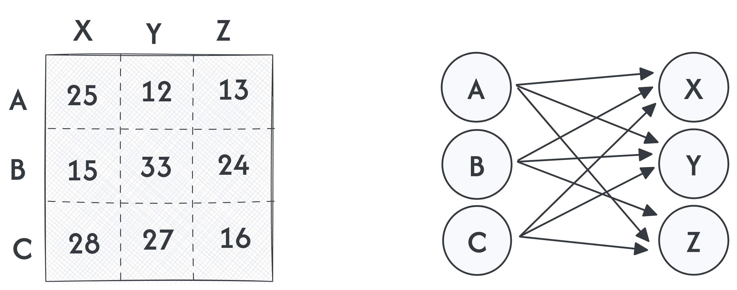 Cost Matrix and its corresponding bipartite graph
In the matrix, the element i-th row and j-th column represents the cost of assigning the job j to company i. The goal is now to minimize the assignment cost. In the example above that would the following.
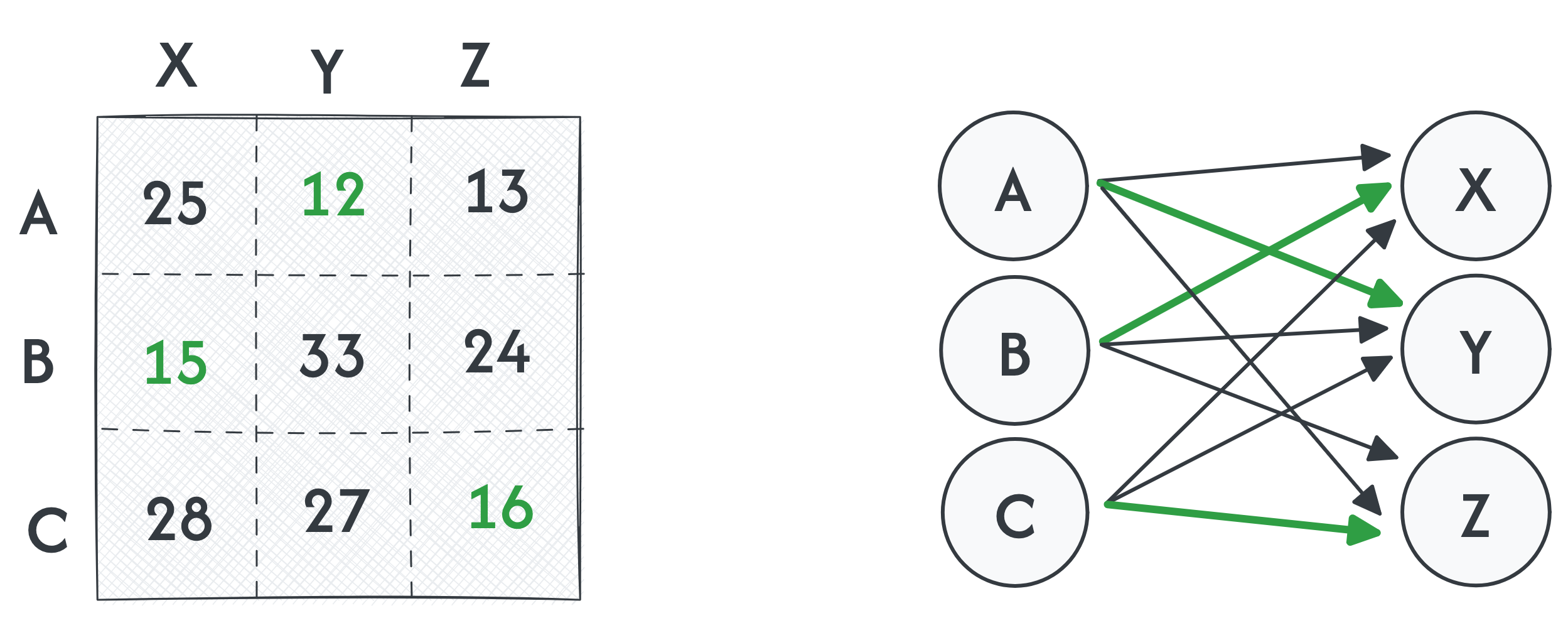 Optimal assignment
This can be also expressed as search for minimal trace of the permuted cost matrix $PC$ by permuting the rows by a permutation matrix $P$.
\[\min_P \text{Trace}(PC)\]There are various formulations of this problem. If we look at the given example, we look for a Minimum Cost Perfect matching, we work with bipartite graph $G$, for which $|U| = |V|$ holds. Formulation for the bipartite graph representation is equivalent, as we look for perfect matching with a minimum assignment cost. Perfect matching means, that each vertex from $U$ is matched against some vertex from $V$. For vertices from both $U$ and $V$ holds, that they have exactly 1 edge assigned to them.
We can further generalize this problem to a scenario in which we are looking for Minimum Cost Matching. In this problem setting, we may have sets of vertices of different cardinalities and we look for complete assignment of workers to jobs.
The Hungarian Algorithm
The Hungarian Algorithm solves the assignment problem by transforming the cost matrix to make optimal assignments easier. It works in the following steps:
- Prepare the Cost Matrix – If the problem is unbalanced, pad the matrix to make it square.
- Reduce Rows and Columns – Subtract the smallest value in each row and column to create zeros in the matrix.
- Cover Zeros – Use the minimum number of horizontal and vertical lines to cover all zeros.
- Adjust the Matrix – If fewer than $n$ lines are needed, modify the matrix by shifting values to create new zeros.
- Find the Optimal Assignment – Select zeros such that each row and column gets exactly one assignment, ensuring minimum total cost.
The minimal cost solution can be described by indices of rows and columns of the cost matrix, that lead to the optimal assignment. The algorithm efficiently finds the matching with the lowest total cost in $O(n^3)$ time, where $n$ is the number of vertices in the larger set of the bipartite graph. Solver for the optimal assignments are well implemented and doesn’t require a lot of work. It’s literally a function call on the cost matrix. The challenging part is to come with a good cost matrix that describes the assignment problem well. In the original DETRtime architecture, the matching is based on a cost matrix $C$, which is a weighted sum 3 cost submatrices.
\[C = w_{CE}*C_{CE} + w_{GIoU}*C_{GIoU} + w_{L1}*C_{L1}\]where
- $C_{GIoU}$ is submatrix of General Intersection over Union for each prediction and target of “the best” box by non-maxima supression.
- $C_{L1}$ is L1 distances of predicted boxes and target boxes,
- Cross Entropy on eye event.
Since the number of predicted objects $N$ is much bigger than the number of ground truth objects, we pad objects by $\emptyset$ (no-object) to produce bipartite matching as desribed in the first step of the algorithm. The optimal matches can then described as the following optimization finding the optimal indices $\hat\theta$ solved by the hungarian algorithm.
\[\hat\theta = \underset{\theta \in \Theta}{\arg\min}\sum_i^N \ell_{match} (y_i, \hat y_{\theta(i)})\]Here, the $\ell_{match}$ is a pair-wise matching cost, ie. the entries in the cost matrix C. The optimal assignment can be computed using the Hungarian algorithm.
Back to Machine Learning
Now that we have the optimal assignment, we can compute the loss function (Hungarian Loss) for all matched pairs. The Hungarian loss specifically in DETRtime is formulated as
\[\ell_{Hungarian} (y, \hat y) = \sum_{i=1}^N \left( -\ln \hat p_{\hat\theta(i)} (c_i) + \mathbb{I}_{\{ c_i \neq \emptyset \}} \cdot \ell_{box} (b_i, \hat b_\theta(i)) \right),\]where
- $\hat p_{\theta (i)} (c_i)$ - probability of class $c_i$
- $\hat \theta$ are the optimal assignment indices
- $\ell_{box}$ - bounding box score
The bounding box score $\ell_{box}$ is a combination of $\ell_1$ and generalized IoU loss $\ell_{IoU}$. This is a good a approach because IoU is scale invariant as opposed to $\ell_1$.
\[\ell_{box} (b_i, \hat b_{\theta(i)}) = \lambda_{IoU}\cdot\ell_{IoU}(b_i, \hat b_{\theta (i)}) + \lambda_{L1} \cdot \|b_i - \hat b_{\theta(i)}\|_1\]where $\lambda$’s are tunable hyperparameters.